Chapter 02 summary
A synopsys of chapter 02 of book "Deep Learning with PyTorch".
Playning with Pretrained models in PyTorch
What is a pretrained model?
- We can think of a pretrained neural network as similar to a program that takes inputs and generates outputs. The behavior of such a program is dictated by the architecture of the neural network and by the examples it saw during training, in terms of desired input-output pairs, or desired properties that the output should satisfy.
We will explore three popular pretrained models: a model that can label an image according to its content, another that can fabricate a new image from a real image, and a model that can describe the content of an image using proper English sentences.
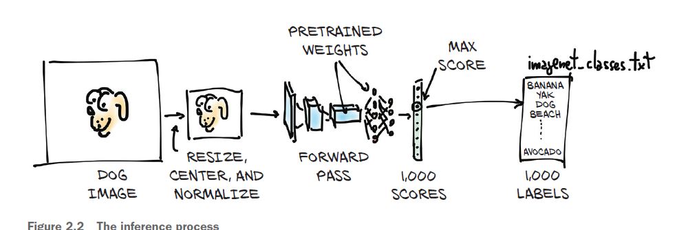
The scope of this chapter is only how to run a pretrained model using PyTorch is a useful skill—full stop. Basically We are going to take our own images and feed them into our pretrained model, as described in figure below. This will result in a list of predicted labels for that image, which we can then examine to see what the model thinks our image is. Some images will have predictions that are accurate, and others will not!
Obtaining a pretrained network for image recognition
The predefined models can be found in torchvision.models
from torchvision import models
We can take a look at the actual models:
dir(models)
['AlexNet',
 'DenseNet',
 'GoogLeNet',
 'GoogLeNetOutputs',
 'Inception3',
 'InceptionOutputs',
 'MNASNet',
 'MobileNetV2',
 'MobileNetV3',
 'ResNet',
 'ShuffleNetV2',
 'SqueezeNet',
 'VGG',
 '_GoogLeNetOutputs',
 .........]
The AlexNet architecture won the 2012 ILSVRC by a large margin, with a top-5 test error rate (that is, the correct label must be in the top 5 predictions) of 15.4%. By comparison, the second-best submission, which wasn’t based on a deep network, trailed at 26.2%. This was a defining moment in the history of computer vision: the moment when the community started to realize the potential of deep learning for vision tasks. That leap was followed by constant improvement, with more modern architectures and training methods getting top-5 error rates as low as 3%.
alexnet = models.AlexNet()
At this point, alexnet is an object that can run the AlexNet architecture.Practically speaking, assuming we have an input object of the right type, we can run the forward pass with output = alexnet(input). But if we did that, we would be feeding data through the whole network to produce … garbage! That’s because the network is uninitialized: its weights, the numbers by which inputs are added and multiplied, have not been trained on anything—the network itself is a blank (or rather, random) slate. We’d need to either train it from scratch or load weights from prior training, which we’ll do now. We learned that the uppercase names correspond to classes that implement popular architectures for computer vision. The lowercase names, on the other hand, are functions that instantiate models with predefined numbers of layers and units and optionally download and load pretrained weights into them. Note that there’s nothing essential about using one of these functions: they just make it convenient to instantiate the model with a number of layers and units that matches how the pretrained networks were built
Let’s create an instance of the network now. We’ll pass an argument that will instruct the function to download the weights of resnet101 trained on the ImageNet dataset, with 1.2 million images and 1,000 categories:
resnet = models.resnet101(pretrained=True)
Downloading: "https://download.pytorch.org/models/resnet101-63fe2227.pth" to C:\Users\hp/.cache\torch\hub\checkpoints\resnet101-63fe2227.pth
100.0%
resnet
ResNet(
  (conv1): Conv2d(3, 64, kernel_size=(7, 7), stride=(2, 2), padding=(3, 3), bias=False)
  (bn1): BatchNorm2d(64, eps=1e-05, momentum=0.1, affine=True, track_running_stats=True)
  (relu): ReLU(inplace)
  (maxpool): MaxPool2d(kernel_size=3, stride=2, padding=1, dilation=1, ceil_mode=False)
  (layer1): Sequential(
    (0): Bottleneck(
      (conv1): Conv2d(64, 64, kernel_size=(1, 1), stride=(1, 1), bias=False)
      (bn1): BatchNorm2d(64, eps=1e-05, momentum=0.1, affine=True, track_running_stats=True)
      (conv2): Conv2d(64, 64, kernel_size=(3, 3), stride=(1, 1), padding=(1, 1), bias=False)
      (bn2): BatchNorm2d(64, eps=1e-05, momentum=0.1, affine=True, track_running_stats=True)
      (conv3): Conv2d(64, 256, kernel_size=(1, 1), stride=(1, 1), bias=False)
      (bn3): BatchNorm2d(256, eps=1e-05, momentum=0.1, affine=True, track_running_stats=True)
      (relu): ReLU(inplace)
      (downsample): Sequential(
        (0): Conv2d(64, 256, kernel_size=(1, 1), stride=(1, 1), bias=False)
        (1): BatchNorm2d(256, eps=1e-05, momentum=0.1, affine=True, track_running_stats=True)
      )
    )
    (1): Bottleneck(
      (conv1): Conv2d(256, 64, kernel_size=(1, 1), stride=(1, 1), bias=False)
      (bn1): BatchNorm2d(64, eps=1e-05, momentum=0.1, affine=True, track_running_stats=True)
      (conv2): Conv2d(64, 64, kernel_size=(3, 3), stride=(1, 1), padding=(1, 1), bias=False)
      (bn2): BatchNorm2d(64, eps=1e-05, momentum=0.1, affine=True, track_running_stats=True)
      (conv3): Conv2d(64, 256, kernel_size=(1, 1), stride=(1, 1), bias=False)
      (bn3): BatchNorm2d(256, eps=1e-05, momentum=0.1, affine=True, track_running_stats=True)
      (relu): ReLU(inplace)
    )
    )
  )
  (avgpool): AvgPool2d(kernel_size=7, stride=1, padding=0)
  (fc): Linear(in_features=2048, out_features=1000, bias=True)
)
What we are seeing here is modules, one per line. Note that they have nothing in common with Python modules: they are individual operations, the building blocks of a neural network. They are also called layers in other deep learning frameworks. If we scroll down, we’ll see a lot of Bottleneck modules repeating one after the other (101 of them!), containing convolutions and other modules. That’s the anatomy of a typical deep neural network for computer vision: a more or less sequential cascade of filters and nonlinear functions, ending with a layer (fc) producing scores for each of the 1,000 output classes (out_features). The resnet variable can be called like a function, taking as input one or more images and producing an equal number of scores for each of the 1,000 ImageNet classes. Before we can do that, however, we have to preprocess the input images so they are the right size and so that their values (colors) sit roughly in the same numerical range. In order to do that, the torchvision module provides transforms, which allow us to quickly define pipelines of basic preprocessing functions:
from torchvision import transforms
preprocess = transforms.Compose([
        transforms.Resize(256),
        transforms.CenterCrop(224),
        transforms.ToTensor(),
        transforms.Normalize(
            mean=[0.485, 0.456, 0.406],
            std=[0.229, 0.224, 0.225]
        )])
In this case, we defined a preprocess function that will scale the input image to 256 × 256, crop the image to 224 × 224 around the center, transform it to a tensor (a PyTorch multidimensional array: in this case, a 3D array with color, height, and width), and normalize its RGB (red, green, blue) components so that they have defined means and standard deviations. These need to match what was presented to the network during training, if we want the network to produce meaningful answers
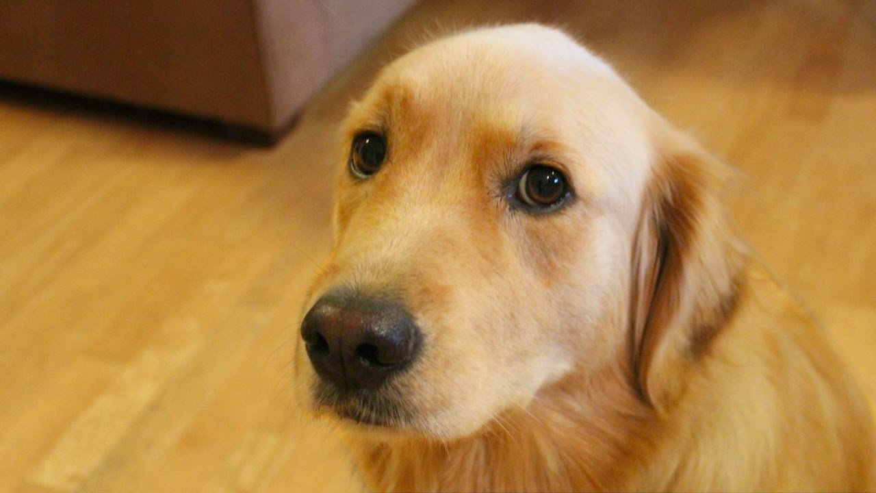
Let’s open a image and visualize it.
from PIL import Image
img = Image.open("../data/p1ch2/bobby.jpg")
img
And do the required preprocessing so that we can use it for prediction from our loaded pretrained model.
img_t = preprocess(img)
import torch
batch_t = torch.unsqueeze(img_t, 0)
The process of running a trained model on new data is called inference in deep learning circles. In order to do inference, we need to put the network in eval mode:
resnet.eval()
ResNet(
  (conv1): Conv2d(3, 64, kernel_size=(7, 7), stride=(2, 2), padding=(3, 3), bias=False)
  (bn1): BatchNorm2d(64, eps=1e-05, momentum=0.1, affine=True, track_running_stats=True)
  (relu): ReLU(inplace=True)

  (avgpool): AdaptiveAvgPool2d(output_size=(1, 1))
  (fc): Linear(in_features=2048, out_features=1000, bias=True)
)
If we forget to do that, some pretrained models, like batch normalization and dropout, will not produce meaningful answers, just because of the way they work internally. Now that eval has been set, we’re ready for inference:
out = resnet(batch_t)
out
  return torch.max_pool2d(input, kernel_size, stride, padding, dilation, ceil_mode)
tensor([[-3.4997e+00, -1.6490e+00, -2.4391e+00, -3.2243e+00, -3.2465e+00,
         -........  4.4534e+00]],
       grad_fn=<AddmmBackward>)
We now need to find out the label of the class that received the highest score. This will tell us what the model saw in the image. If the label matches how a human would describe the image, that’s great! It means everything is working. If not, then either something went wrong during training, or the image is so different from what the model expects that the model can’t process it properly, or there’s some other similar issue.
Let’s load the file containing the 1,000 labels for the ImageNet dataset classes:
with open('../data/p1ch2/imagenet_classes.txt') as f:
    labels = [line.strip() for line in f.readlines()]
_, index = torch.max(out, 1)
percentage = torch.nn.functional.softmax(out, dim=1)[0] * 100
labels[index[0]], percentage[index[0]].item()
('golden retriever', 96.57185363769531)
_, indices = torch.sort(out, descending=True)
[(labels[idx], percentage[idx].item()) for idx in indices[0][:5]]
[('golden retriever', 96.57185363769531),
 ('Labrador retriever', 2.6082706451416016),
 ('cocker spaniel, English cocker spaniel, cocker', 0.2699621915817261),
 ('redbone', 0.17958936095237732),
 ('tennis ball', 0.10991999506950378)]
We see that the first four are dogs (redbone is a breed; who knew?), after which things start to get funny. The fifth answer, “tennis ball,” is probably because there are enough pictures of tennis balls with dogs nearby that the model is essentially saying, “There’s a 0.1% chance that I’ve completely misunderstood what a tennis ball is.” This is a great example of the fundamental differences in how humans and neural networks view the world, as well as how easy it is for strange, subtle biases to sneak into our data.